Place names in Alsace

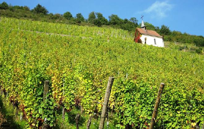
Names of places in Alsace are sometimes described as unpronounceable for French people. Most names have a Germanic root and sound pretty exotic for French speakers. I recommend taking a regional train and listening to the voice announcing the Alsatian stations with a very French pronunciation, quite a funny experience. A recent trip on the train made me think about the similarity of suffixes in Alsatian place names and I was interested to know how many places actually end on “-heim”, “-willer” and so on.

This post uses data from a scraped Wikipedia table from another post. It contains information on communes in the département Bas-Rhin. Here, we only need the names of the places. We start by loading packages, data and pulling out the column we are interested in.

# Load packages
library(tidyverse)
library(sylly)

# Load data
bas_rhin <- read_csv("https://dwitkowski.eu/assets/data/bas_rhin.csv")

# Get name column
bas_rhin_noms <- bas_rhin %>%
  filter(nom != "Bas-Rhin") %>%
  pull(nom)

First thing to clean up is possible extensions of the place names, such as river names (e.g. -sur-Zorn or -les-Bains).

bas_rhin_noms <- str_split(bas_rhin_noms, "-") %>%
  map_chr(tail(1))

As we are interested in the suffixes of the place names, we need a method to split the strings into syllables. We will use the method hyphen() from the sylly package that takes vectors of character strings and applies an hyphenation algorithm to each word (the algorithm was originally developed for automatic word hyphenation in LaTeX). The algorithm needs a set of hyphenation patterns which are provided in dictionaries for different languages. Let’s try out the French (Alsace is in France!) and German (Alsatian is a German dialect) dictionaries for the place names.

# Define dictionary for syllables
## French
url.fr.pattern <- url("http://tug.ctan.org/tex-archive/language/hyph-utf8/tex/generic/hyph-utf8/patterns/txt/hyph-fr.pat.txt")
hyph.fr <- read.hyph.pat(url.fr.pattern, lang="fr")
close(url.fr.pattern)

## German
url.de.pattern <- url("http://tug.ctan.org/tex-archive/language/hyph-utf8/tex/generic/hyph-utf8/patterns/txt/hyph-de-1996.pat.txt")
hyph.de <- read.hyph.pat(url.de.pattern, lang="de")
close(url.de.pattern)

# Split into syllables
## based on French dictionary
syllables_fr <- hyphen(bas_rhin_noms, hyph.pattern=hyph.fr) %>%
  hyphenText() %>%
  mutate(id = row_number()) %>%
  select(id, french = word)

## based on German dictionary
syllables_de <- hyphen(bas_rhin_noms, hyph.pattern=hyph.de) %>%
  hyphenText() %>%
  mutate(id = row_number()) %>%
  select(id, german = word)

# Merge data sets
syllables <- left_join(syllables_fr, syllables_de, by = "id")

# Compare the syllables based on the two dictionaries
syllables %>%
  count(french == german)

# A tibble: 2 x 2
  `french == german`     n
  <lgl>              <int>
1 FALSE                258
2 TRUE                 255

There are 255 names split in the same way, 258 differently. Indeed, the choice of the dictionary affects the outcomes. After manually inspecting the differences, I opt for the German dictionary because it splits syllables better than the French one for the names under study (e.g. -heim vs. -sheim, e.g. -wil-ler vs. -swiller).

However, there are still some manual corrections necessary, for example reuniting some syllables (like -wil and -ler) to get the correct suffixes.

syllables_de <- syllables_de %>%
  mutate(german = str_replace_all(german,
                            c("wil-ler" = "willer",
                              "hof-fen" = "hoffen",
                              "hou-sen" = "housen",
                              "hau-sen" = "hausen",
                              "mun-ster" = "munster",
                              "kir-chen" = "kirchen",
                              "ber-gen" = "bergen",
                              "sheim" = "heim",
                              "zheim" = "heim",
                              "schwiller" = "willer",
                              "dertheim" = "heim"))) %>%
  pull(german)

Now we are ready to extract the suffix and count their appearences.

# Extract suffix
suffixes <- str_split(syllables_de, "-") %>%
  sapply(tail, 1)

# Tidy and count suffixes
suffixes <- enframe(suffixes) %>%
  # drop obs which had only one syllable left (start with capital letter)
  filter(!str_detect(value, "^[A-Z]")) %>%
  # Count values
  count(value) %>%
  # Calculate proportion
  mutate(percent = n / cumsum(n)[length(n)]) %>%
  # Add a hyphen in beginning of suffix
  mutate(value = str_c("-", value)) %>%
  # Change suffix to factor (for correct order in bar chart)
  mutate(suffix = factor(value, levels = value[order(n)])) %>%
  # Sort data
  select(suffix, n, percent, -value) %>%  
  arrange(desc(n))

# Show 10 most common suffixes
head(suffixes, 10)

# A tibble: 10 x 3
   suffix      n percent
   <fct>   <int>   <dbl>
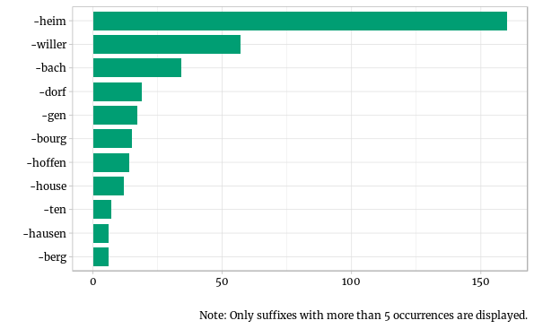
 1 -heim     160  0.342
 2 -willer    57  0.122
 3 -bach      34  0.0726
 4 -dorf      19  0.0406
 5 -gen       17  0.0363
 6 -bourg     15  0.0321
 7 -hoffen    14  0.0299
 8 -house     12  0.0256
 9 -ten        7  0.0150
10 -berg       6  0.0128

By far, the most common suffix in place names in Bas-Rhin is “-heim” (cf. also the graph below). More than a third of all the communes have this suffix. Other common suffixes are “-willer” (12%), “-bach” (7%), and “-dorf” (4%). As a last piece, here’s a bar chart visualizing this information.

# Visualize data
ggplot(data = filter(suffixes, n > 5)) +
  geom_bar(aes(x = suffix, y = n), width = 0.8, fill = "#009E73", stat = "identity") +
  coord_flip() +
  theme_light() +
  theme(text = element_text(family = "serif"),
        axis.text.x = element_text(color = "black"),
        axis.text.y = element_text(color = "black")) +
  xlab("") +
  ylab("") +
  labs(caption = "Only suffixes with more than 5 occurrences are displayed.")

This analysis was limited to places in the département Bas-Rhin, but I might extend it to the second Alsatian département Haut-Rhin in the near future.

Get the code here.